Benchmarks
Regroup typical EC benchmarks functions to import easily and benchmark examples.
| Single Objective Continuous | Multi Objective Continuous | Binary | Symbolic Regression |
|---|---|---|---|
cigar() |
fonseca() |
chuang_f1() |
kotanchek() |
plane() |
kursawe() |
chuang_f2() |
salustowicz_1d() |
sphere() |
schaffer_mo() |
chuang_f3() |
salustowicz_2d() |
rand() |
dtlz1() |
royal_road1() |
unwrapped_ball() |
ackley() |
dtlz2() |
royal_road2() |
rational_polynomial() |
bohachevsky() |
dtlz3() |
rational_polynomial2() |
|
griewank() |
dtlz4() |
sin_cos() |
|
h1() |
zdt1() |
ripple() |
|
himmelblau() |
zdt2() |
||
rastrigin() |
zdt3() |
||
rastrigin_scaled() |
zdt4() |
||
rastrigin_skew() |
zdt6() |
||
rosenbrock() |
|||
schaffer() |
|||
schwefel() |
|||
shekel() |
Continuous Optimization
-
deap.benchmarks.cigar(individual)[source]¶ Cigar test objective function.
Type minimization Range none Global optima 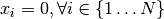 ,
, 
Function 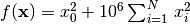
-
deap.benchmarks.plane(individual)[source]¶ Plane test objective function.
Type minimization Range none Global optima , Function 
-
deap.benchmarks.sphere(individual)[source]¶ Sphere test objective function.
Type minimization Range none Global optima , Function 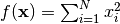
-
deap.benchmarks.rand(individual)[source]¶ Random test objective function.
Type minimization or maximization Range none Global optima none Function 
-
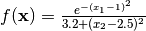
deap.benchmarks.ackley(individual)[source]¶ Ackley test objective function.
Type minimization Range ![x_i \in [-15, 30]](../_images/math/44175b2140f0c059455a78a1ca11a73be3772088.png)
Global optima , Function 
-
deap.benchmarks.bohachevsky(individual)[source]¶ Bohachevsky test objective function.
Type minimization Range ![x_i \in [-100, 100]](../_images/math/2a3df0cc70f044e065ff87fb71ed2b4db0f5bae6.png)
Global optima , Function 
-
deap.benchmarks.griewank(individual)[source]¶ Griewank test objective function.
Type minimization Range ![x_i \in [-600, 600]](../_images/math/20de17eec0b7d3e331aa285c01849f4f4977e864.png)
Global optima , Function 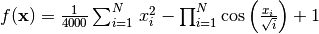
-
deap.benchmarks.h1(individual)[source]¶ Simple two-dimensional function containing several local maxima. From: The Merits of a Parallel Genetic Algorithm in Solving Hard Optimization Problems, A. J. Knoek van Soest and L. J. R. Richard Casius, J. Biomech. Eng. 125, 141 (2003)
Type maximization Range Global optima  ,
, 
Function 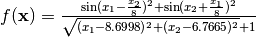
-
deap.benchmarks.himmelblau(individual)[source]¶ The Himmelblau’s function is multimodal with 4 defined minimums in
![[-6, 6]^2](../_images/math/a142b2ffef1a69524aa943205e71b264ce95e556.png) .
.Type minimization Range ![x_i \in [-6, 6]](../_images/math/ffa194e8b4edc477b466f988087269702392c27d.png)
Global optima  ,
, 
 ,
, 
 ,
, 
 ,
, 
Function 
-
deap.benchmarks.rastrigin(individual)[source]¶ Rastrigin test objective function.
Type minimization Range ![x_i \in [-5.12, 5.12]](../_images/math/4619ad3bf5c5afcbbb92ce45ef7e2f2e2d2fa137.png)
Global optima , Function 


-
deap.benchmarks.rosenbrock(individual)[source]¶ Rosenbrock test objective function.
Type minimization Range none Global optima  ,
, Function 
-
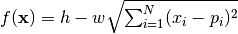
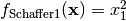
deap.benchmarks.schaffer(individual)[source]¶ Schaffer test objective function.
Type minimization Range Global optima , Function ![f(\mathbf{x}) = \sum_{i=1}^{N-1} (x_i^2+x_{i+1}^2)^{0.25} \cdot \left[ \sin^2(50\cdot(x_i^2+x_{i+1}^2)^{0.10}) + 1.0 \right]](../_images/math/fccb4296e58b381cb783fbffeb0feaf93436454f.png)
-
deap.benchmarks.schwefel(individual)[source]¶ Schwefel test objective function.
Type minimization Range ![x_i \in [-500, 500]](../_images/math/77d204f4021b0775cbd8fc98f73bc5bb548285ec.png)
Global optima  ,
, Function 
-
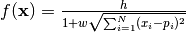
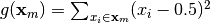
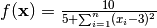
deap.benchmarks.shekel(individual, a, c)[source]¶ The Shekel multimodal function can have any number of maxima. The number of maxima is given by the length of any of the arguments a or c, a is a matrix of size
 , where M is the number of maxima
and N the number of dimensions and c is a
, where M is the number of maxima
and N the number of dimensions and c is a  vector.
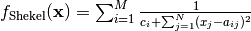
The following figure uses
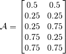 and
and
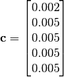 , thus defining 5 maximums in
 .
.
Multi-objective
-
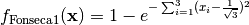
deap.benchmarks.fonseca(individual)[source]¶ Fonseca and Fleming’s multiobjective function. From: C. M. Fonseca and P. J. Fleming, “Multiobjective optimization and multiple constraint handling with evolutionary algorithms – Part II: Application example”, IEEE Transactions on Systems, Man and Cybernetics, 1998.


-
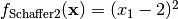
deap.benchmarks.schaffer_mo(individual)[source]¶ Schaffer’s multiobjective function on a one attribute individual. From: J. D. Schaffer, “Multiple objective optimization with vector evaluated genetic algorithms”, in Proceedings of the First International Conference on Genetic Algorithms, 1987.
-
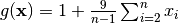
deap.benchmarks.dtlz1(individual, obj)[source]¶ DTLZ1 multiobjective function. It returns a tuple of obj values. The individual must have at least obj elements. From: K. Deb, L. Thiele, M. Laumanns and E. Zitzler. Scalable Multi-Objective Optimization Test Problems. CEC 2002, p. 825 - 830, IEEE Press, 2002.


Where
 is the number of objectives and
  is a
vector of the remaining attributes
is a
vector of the remaining attributes ![[x_m~\ldots~x_n]](../_images/math/ea6b634a25d6afacfd6102b3c69952b7a0184392.png) of the
individual in
of the
individual in  dimensions.
-
deap.benchmarks.dtlz2(individual, obj)[source]¶ DTLZ2 multiobjective function. It returns a tuple of obj values. The individual must have at least obj elements. From: K. Deb, L. Thiele, M. Laumanns and E. Zitzler. Scalable Multi-Objective Optimization Test Problems. CEC 2002, p. 825 - 830, IEEE Press, 2002.


Where
is the number of objectives and is a
vector of the remaining attributes of the
individual in dimensions.
-
deap.benchmarks.dtlz3(individual, obj)[source]¶ DTLZ3 multiobjective function. It returns a tuple of obj values. The individual must have at least obj elements. From: K. Deb, L. Thiele, M. Laumanns and E. Zitzler. Scalable Multi-Objective Optimization Test Problems. CEC 2002, p. 825 - 830, IEEE Press, 2002.


Where
is the number of objectives and is a
vector of the remaining attributes of the
individual in dimensions.
-
deap.benchmarks.dtlz4(individual, obj, alpha)[source]¶ DTLZ4 multiobjective function. It returns a tuple of obj values. The individual must have at least obj elements. The alpha parameter allows for a meta-variable mapping in
dtlz2() , the authors suggest
  .
From: K. Deb, L. Thiele, M. Laumanns and E. Zitzler. Scalable Multi-Objective
Optimization Test Problems. CEC 2002, p. 825 - 830, IEEE Press, 2002.
.
From: K. Deb, L. Thiele, M. Laumanns and E. Zitzler. Scalable Multi-Objective
Optimization Test Problems. CEC 2002, p. 825 - 830, IEEE Press, 2002.


Where
is the number of objectives and is a
vector of the remaining attributes of the
individual in dimensions.
![f_{\text{ZDT1}2}(\mathbf{x}) = g(\mathbf{x})\left[1 - \sqrt{\frac{x_1}{g(\mathbf{x})}}\right]](../_images/math/918cc1f17fb5161281b597488cef612ee41d1486.png)
![f_{\text{ZDT2}2}(\mathbf{x}) = g(\mathbf{x})\left[1 - \left(\frac{x_1}{g(\mathbf{x})}\right)^2\right]](../_images/math/5459ed3625b34cc1683f15a01ec1cddb2aedadd6.png)
![f_{\text{ZDT3}2}(\mathbf{x}) = g(\mathbf{x})\left[1 - \sqrt{\frac{x_1}{g(\mathbf{x})}} - \frac{x_1}{g(\mathbf{x})}\sin(10\pi x_1)\right]](../_images/math/6394bbe3cfd248aedc6a20936a36c1fe8c39c3eb.png)
![g(\mathbf{x}) = 1 + 10(n-1) + \sum_{i=2}^n \left[ x_i^2 - 10\cos(4\pi x_i) \right]](../_images/math/045f34eb3e79fb91fd129ae36aa9d704d0fa4b57.png)
![f_{\text{ZDT4}2}(\mathbf{x}) = g(\mathbf{x})\left[ 1 - \sqrt{x_1/g(\mathbf{x})} \right]](../_images/math/962562e6f4092e2717a413f89e657708d722351c.png)
![g(\mathbf{x}) = 1 + 9 \left[ \left(\sum_{i=2}^n x_i\right)/(n-1) \right]^{0.25}](../_images/math/cee16ca7f6cb950698224c4ff202d7d2f0773b2e.png)

![f_{\text{ZDT6}2}(\mathbf{x}) = g(\mathbf{x}) \left[ 1 - (f_{\text{ZDT6}1}(\mathbf{x})/g(\mathbf{x}))^2 \right]](../_images/math/2f66cdda39d5ef6fb0fd3eff6ac711ac9364f0cd.png)
Binary Optimization
-
deap.benchmarks.binary.chuang_f1(individual)[source]¶ Binary deceptive function from : Multivariate Multi-Model Approach for Globally Multimodal Problems by Chung-Yao Chuang and Wen-Lian Hsu.
The function takes individual of 40+1 dimensions and has two global optima in [1,1,…,1] and [0,0,…,0].
-
deap.benchmarks.binary.chuang_f2(individual)[source]¶ Binary deceptive function from : Multivariate Multi-Model Approach for Globally Multimodal Problems by Chung-Yao Chuang and Wen-Lian Hsu.
The function takes individual of 40+1 dimensions and has four global optima in [1,1,…,0,0], [0,0,…,1,1], [1,1,…,1] and [0,0,…,0].
-
deap.benchmarks.binary.chuang_f3(individual)[source]¶ Binary deceptive function from : Multivariate Multi-Model Approach for Globally Multimodal Problems by Chung-Yao Chuang and Wen-Lian Hsu.
The function takes individual of 40+1 dimensions and has two global optima in [1,1,…,1] and [0,0,…,0].
-
deap.benchmarks.binary.royal_road1(individual, order)[source]¶ Royal Road Function R1 as presented by Melanie Mitchell in : “An introduction to Genetic Algorithms”.
Symbolic Regression
![\mathbf{x} \in [-1, 7]^2](../_images/math/d88a9d922d10b7e1246a30bbb6d38d12e2200886.png)
![x \in [0, 10]](../_images/math/56d969426d71335644a40028d8a3d995fd291eba.png)

![\mathbf{x} \in [0, 7]^2](../_images/math/3e75e385920a4c0ed8e9140a6675783c4c904cc0.png)

![\mathbf{x} \in [-2, 8]^n](../_images/math/0156220a78f8262c07caae91841067b72776c2db.png)
-
deap.benchmarks.gp.rational_polynomial(data)[source]¶ Rational polynomial ball benchmark function.
Range ![\mathbf{x} \in [0, 2]^3](../_images/math/8d9ddb039e1a628b5f4111e3955e09ac14246dba.png)
Function 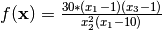
![\mathbf{x} \in [0, 6]^2](../_images/math/21b9304388c5e350b04df4b2b31835a519d69fbd.png)

![\mathbf{x} \in [-5, 5]^2](../_images/math/b637f7b1e17344cbcb6d0ff572fdca01979f06d6.png)

Moving Peaks Benchmark
Re-implementation of the Moving Peaks Benchmark by Jurgen Branke. With the addition of the fluctuating number of peaks presented in du Plessis and Engelbrecht, 2013, Self-Adaptive Environment with Fluctuating Number of Optima.
-
class
deap.benchmarks.movingpeaks.MovingPeaks(self, dim[, pfunc][, npeaks][, bfunc][, random][, ...])[source]¶ The Moving Peaks Benchmark is a fitness function changing over time. It consists of a number of peaks, changing in height, width and location. The peaks function is given by pfunc, wich is either a function object or a list of function objects (the default is
function1()). The number of peaks is determined by npeaks (which defaults to 5). This parameter can be either a integer or a sequence. If it is set to an integer the number of peaks won’t change, while if set to a sequence of 3 elements, the number of peaks will fluctuate between the first and third element of that sequence, the second element is the inital number of peaks. When fluctuating the number of peaks, the parameter number_severity must be included, it represents the number of peak fraction that is allowed to change. The dimensionality of the search domain is dim. A basis function bfunc can also be given to act as static landscape (the default is no basis function). The argument random serves to grant an independent random number generator to the moving peaks so that the evolution is not influenced by number drawn by this object (the default uses random functions from the Python modulerandom). Various other keyword parameters listed in the table below are required to setup the benchmark, default parameters are based on scenario 1 of this benchmark.Parameter SCENARIO_1(Default)SCENARIO_2SCENARIO_3Details pfuncfunction1()cone()cone()The peak function or a list of peak function. npeaks5 10 50 Number of peaks. If an integer, the number of peaks won’t change, if a sequence it will fluctuate [min, current, max]. bfuncNoneNonelambda x: 10Basis static function. min_coord0.0 0.0 0.0 Minimum coordinate for the centre of the peaks. max_coord100.0 100.0 100.0 Maximum coordinate for the centre of the peaks. min_height30.0 30.0 30.0 Minimum height of the peaks. max_height70.0 70.0 70.0 Maximum height of the peaks. uniform_height50.0 50.0 0 Starting height for all peaks, if uniform_height <= 0the initial height is set randomly for each peak.min_width0.0001 1.0 1.0 Minimum width of the peaks. max_width0.2 12.0 12.0 Maximum width of the peaks uniform_width0.1 0 0 Starting width for all peaks, if uniform_width <= 0the initial width is set randomly for each peak.lambda_0.0 0.5 0.5 Correlation between changes. move_severity1.0 1.5 1.0 The distance a single peak moves when peaks change. height_severity7.0 7.0 1.0 The standard deviation of the change made to the height of a peak when peaks change. width_severity0.01 1.0 0.5 The standard deviation of the change made to the width of a peak when peaks change. period5000 5000 1000 Period between two changes. Dictionnaries
SCENARIO_1,SCENARIO_2andSCENARIO_3of this module define the defaults for these parameters. The scenario 3 requires a constant basis function which can be given as a lambda functionlambda x: constant.The following shows an example of scenario 1 with non uniform heights and widths.